This is a practice test I was given prior to landing a contract with the Tampa Bay Rays from July 2021. Here, I was asked to predict hit speed given angle off the bat. There’s a publicly available github repository with the same data here: https://github.com/danhogan/batted-ball. Below is copied from the practice test. This is not technical, and done on a timer. I was asked to discuss a few things, and had to little time to curate content. Any corrections or suggestions to make this more rigorous is helpful, as this is quite casual.
setwd("/home/andre/rays/test/");
dt = read.csv("battedBallData.csv");
require(rstan);
require(psych);
set.seed(1);

## function to standardize real covariates
standardize = function(x) {
  x_mu = mean(x);
  x_sd = sd(x);
  x_std = (x - x_mu) / x_sd;
  return(list(x_std, x_mu, x_sd));
}
Summary
In this work, I use a multilevel Gaussian process model to predict speed, given hit type and angle. The Gaussian process allows us to estimate the functional relationship between angle off bat and speed of bat. Adding multiple levels in the Gaussian process allows us to estimate the different different functional effects for each hittype.
To complete the task, I used system A. After making plots it looked like system B had trouble detecting angles below 20 degrees. This could be a mechanical failure or due to the placement of the machine.. Given more time, it’s possible to combine both scores in a model using some kind of multiple output GP, or averaging over both sets of predictors, given more time.
It’s possible to predict conditional functional relationship at the individual player level using Gaussian processes, but introducing player level intercepts added divergences. was prior to changing the likelihood function to a Cauchy distribution, so this was probably due to over regularization from the Gaussian likelihood, but can be done with more time and fitting more models. Below, I also explain a method for downsampling that can be used to get player-cluster level estimates. In summary, we use a ML-based clustering method to put players together into groups, assuming there exists some batters that bat similarly, and the use these clusters as levels. I review this in more detail later.
I also do some exploratory analysis that mostly consists of histograms and scatterplots, not all of which I include here. It’s important to visualize conditional observed distributions. I.e. angle v speed with different batters, pitchers, and hit type combinations, not all of which I included here.
In the PDF, you also mentioned that you wanted to see how I handled “imperfect data”. Almost no real, observational data is “perfect”. The only real data I’ve seen that was approximately normal was for a clinical trial at UNC. In this case, I just dropped missing observations since we have enough data, and to make the process faster, but I include descriptions and code about how we can integrate out censored observations in a survival model and how we can model missing observations in the covariance matrix in a GP.
Finally, after running many models I include code and results for a finalized multilevel GP regression with a Cauchy likelihood, and functional predictions for hitspeed conditional on each batting type, on a reduced size and larger dataset.
Exploratory Analysis
Investigate Tendencies Within Pitchers
pitchers = unique(dt$pitcher);

## uncomment the following block for some quick exploratory data analysis
N_plots = 50;
for (i in 1:N_plots) {
  dt_p = dt[which(dt$pitcher == pitchers[i]),];
  par(mfrow = c(1,2))
  plot(dt_p$vangle_A, dt_p$speed_A, xlim = c(-70, 70), ylim = c(40, 110), main = as.character(pitchers[i]), col = "#F5D130");
  plot(dt_p$vangle_B, dt_p$speed_B, xlim = c(-70, 70), ylim = c(40, 110), col = "#092C5C");
}
Investigate Tendencies Within Batters
batters = unique(dt$batter);

## uncomment the following block for some quick exploratory data analysis
N_plots = 50;
for (i in 1:N_plots) {
  dt_b = dt[which(dt$batter == batters[i]),];
  par(mfrow = c(1,2))
  plot(dt_b$vangle_A, dt_b$speed_A, xlim = c(-70, 70), ylim = c(40, 110), main = as.character(batters[i]), col = "#F5D130");
  plot(dt_b$vangle_B, dt_b$speed_B, xlim = c(-70, 70), ylim = c(40, 110), col = "#092C5C");
}
I’ve hidden the figures, but you can look at many batting and pitching tendencies by removing the fig.show='hide' command in the previous chunk of code.
Clearly, there’s a general trend that angles father from zero result in lower speed- off-bat (SOB). One trait that separates a good batter from a bad batter is one that is able to have a high SOB independent of the angle. I.E. a pitch low in the batting box, high in the batting box, a good batter will be able to recover this and still have a high SOB. For example, for simplicity if we omit the kind of bat, i.e. fly-ball, which we shouldn’t admit when making a hiring decision, we might judge a good batter by their ability to hit balls at high speeds even at poor angles, poor angle meaning far from 0.
That said, after some exploratory data analysis with the first 50 batters, here’s some batters with that property: High SOB, independent of angle. And here’s some batters we should measure more, by throwing pitches at wild angles to see how they compensate.
Given more time, we’d look at speed/batter/pitcher combos conditional on type of bat it was.
115 is really good. 8 looks good.
dt_b = dt[which(dt$batter == 115),];
par(mfrow = c(1,2))
plot(dt_b$speed_A, dt_b$vangle_A, xlim = c(40, 110), ylim = c(-70, 70), main = as.character(115), col = "#F5D130");
plot(dt_b$speed_B, dt_b$vangle_B, xlim = c(40, 110), ylim = c(-70, 70), col = "#092C5C");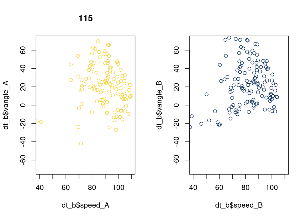
dt_b = dt[which(dt$batter == 8),];
par(mfrow = c(1,2))
plot(dt_b$speed_A, dt_b$vangle_A, xlim = c(40, 110), ylim = c(-70, 70), main = as.character(8), col = "#F5D130");
plot(dt_b$speed_B, dt_b$vangle_B, xlim = c(40, 110), ylim = c(-70, 70), col = "#092C5C");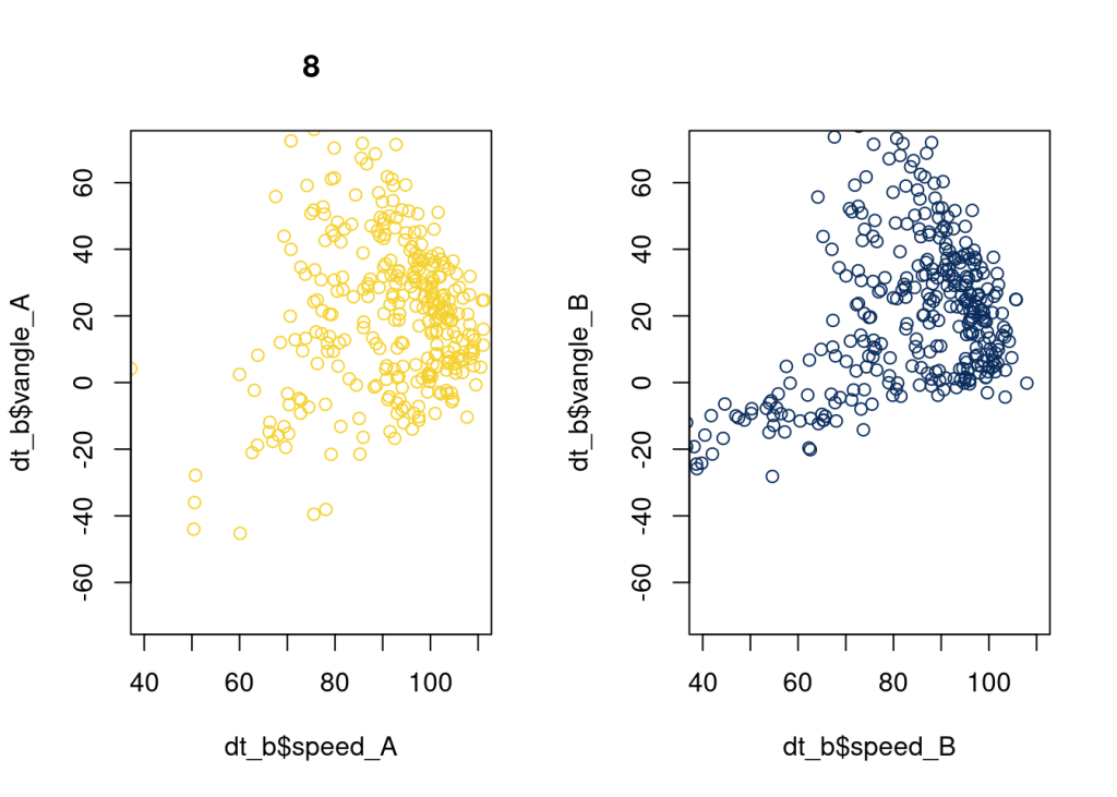
And here’s an example of a batter we’d likely re-weight with a prior closer to the median or mean, but a batter that warrants investigation (i.e. throw more pitches at him at wild angles), since he seems to have a pretty consistently high SOB. We’d like to see if this was signal or just chance.
dt_b = dt[which(dt$batter == 74),];
par(mfrow = c(1,2))
plot(dt_b$speed_A, dt_b$vangle_A, xlim = c(40, 110), ylim = c(-70, 70), main = as.character(74), col = "#F5D130");
plot(dt_b$speed_B, dt_b$vangle_B, xlim = c(40, 110), ylim = c(-70, 70), col = "#092C5C");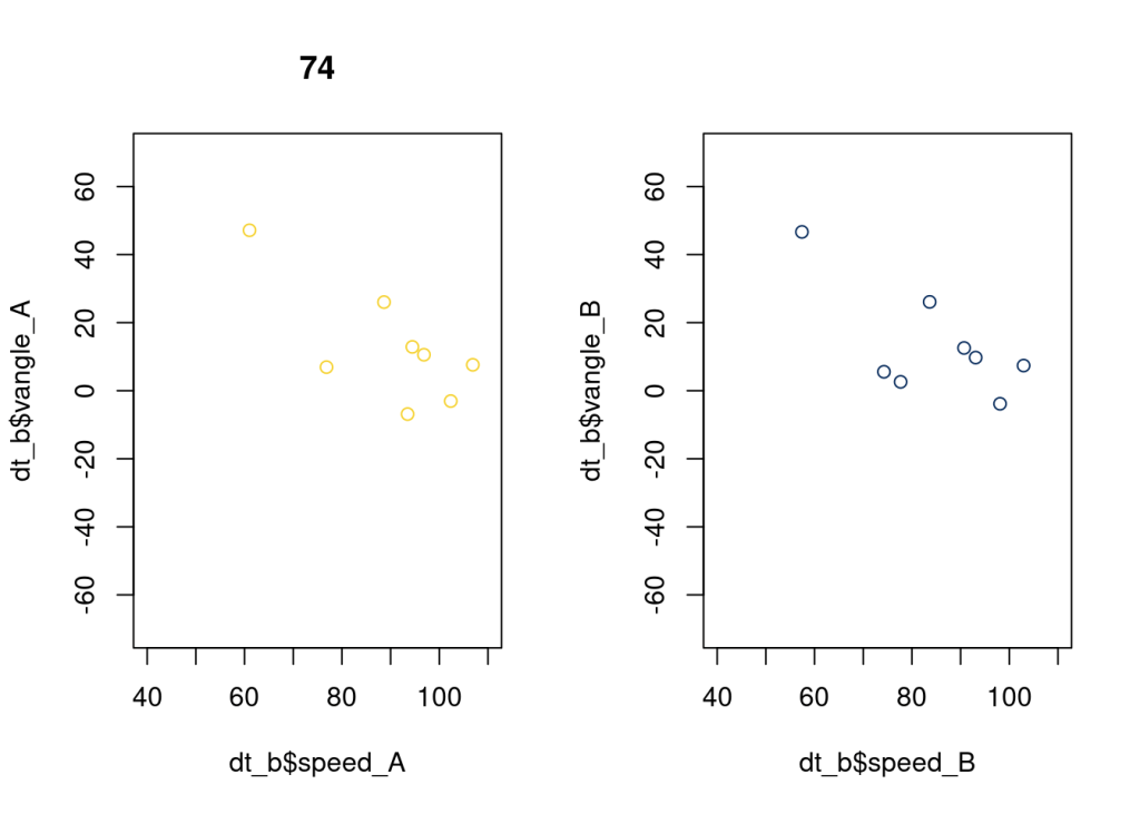
Imperfect Data
There’s missing observations. This happens all the time with real data. Some cases, if the number of observations per group differs, we can go ahead and use a multilevel model, if this is suitable for the given analysis. In the biomed, classical statistics literature, we call these linear mixed effects models. In Bayesian, they’re just multilevel models, since all parameters are “mixed effects”. Since we put priors on these parameters, we call them hierarchical models.
This kind of model doesn’t work in all cases. Suppose we’re trying to model “time to failure” type data, or investigate a risk model when we have data over time. These are called survival models, and are common, for example, cardiology where we’d like to model of myocardial infarction (MCI) and factors that contribute to risk thereof overtime. In survival models, we encounter “missing data” all the time. These are called . There are different types of censorship (right censored), left censored, etc. This discussion
Handling Censored Observations in Stan (and in GP models)
In survival models, and in Bayesian statistics, and in Stan, we don’t throw this data away. We model the censored observations, and integrate them out. The Stan code would look something like this, depending on the model:
target += lognormal_lccdf(y[censored_idx] | f[censored_idx], sigma);This was for an AFT survival model, where the likelihood function used was a loggaussian. Similarly, could have used a Weibull distribution. The ff here was estimated with a GP. Here’s the full Stan code for this survival model. This isn’t the model I’m using for this data, just an example of something I’ve used in the past:
writeLines(readLines("loggaussian_survival_gp.stan"))## functions {
## vector gp_pred_exp_quad_rng(vector[] x_pred,
## vector y1, vector[] x,
## real magnitude, real[] length_scale, real sigma) {
## int N1 = rows(y1);
## int N2 = size(x_pred);
## vector[N2] f2;
## {
## matrix[N1, N1] K = gp_exp_quad_cov(x, magnitude, length_scale)
## + diag_matrix(rep_vector(square(sigma), N1));
## matrix[N1, N1] L_K = cholesky_decompose(K);
##
## vector[N1] L_K_div_y1 = mdivide_left_tri_low(L_K, y1);
## vector[N1] K_div_y1 = mdivide_right_tri_low(L_K_div_y1', L_K)';
## matrix[N1, N2] k_x_x_pred = gp_exp_quad_cov(x, x_pred, magnitude, length_scale);
## vector[N2] f2_mu = (k_x_x_pred' * K_div_y1);
## matrix[N1, N2] v_pred = mdivide_left_tri_low(L_K, k_x_x_pred);
## matrix[N2, N2] cov_f2 = gp_exp_quad_cov(x_pred, magnitude, length_scale) - v_pred' * v_pred
## + diag_matrix(rep_vector(1e-6, N2));
## f2 = multi_normal_rng(f2_mu, cov_f2);
## }
## return f2;
## }
## }
## data {
## int<lower=1> N;
## int<lower=1> D;
## int<lower=1> N_pred;
## int<lower=1> n_events;
## int<lower=0> n_censored;
## vector[D] x[N];
##
## // what we'd like to make predictions for
## vector[D] x_male_age[N_pred];
## vector[D] x_female_age[N_pred];
##
## vector[N] y; // time for observation n
## vector[N] event;
## int event_idx[n_events];
## int censored_idx[n_censored];
## }
##
## transformed data {
## vector[N] y_new = y / exp(mean(log(y)));
## }
## parameters {
## real<lower=0> magnitude;
## real<lower=0> length_scale[D];
## real<lower=0> sig_0;
## real<lower=0> sigma;
## vector[N] eta;
## }
## transformed parameters {
## vector[N] f;
## {
## matrix[N, N] L_K;
## // below is if we want to estimate using linear covariance (i.e. linear model)
## // matrix[N, N] K = gp_dot_prod_cov(x, sig_0) + gp_exp_quad_cov(x, magnitude, length_scale);
## matrix[N, N] K = gp_exp_quad_cov(x, magnitude, length_scale);
## K = add_diag(K, sigma);
## L_K = cholesky_decompose(K);
## f = L_K * eta;
## }
## }
## model {
## length_scale ~ gamma(2, 2);
## magnitude ~ normal(0, 2);
## sig_0 ~ normal(0, 2);
## sigma ~ normal(0, 1);
## eta ~ normal(0, 1);
##
## target += lognormal_lpdf(y[event_idx] | f[event_idx], sigma);
## target += lognormal_lccdf(y[censored_idx] | f[censored_idx], sigma);
## }
## generated quantities {
##
## // conditional posterior for latent f for male, female)
## // using squared exponential covariance function (i.e. it's smooth).
## vector[N_pred] f_male_age = gp_pred_exp_quad_rng(x_male_age, f, x,
## magnitude, length_scale, sigma);
## vector[N_pred] f_female_age = gp_pred_exp_quad_rng(x_female_age, f, x,
## magnitude, length_scale, sigma);
##
## // conditional posterior predictive distribution.
## vector[N_pred] y_male_age;
## vector[N_pred] y_female_age;
## for (n in 1:N_pred) {
## y_male_age[n] = lognormal_rng(f_male_age[n], sigma);
## y_female_age[n] = lognormal_rng(f_female_age[n], sigma);
## }
## }With Gaussian processes, if we’re not using a survival model, we can model the censored observations in the covariance matrix, i.e. the covariance between a censored observation on one dimension and another is 0. Really, modeling censored observations depends on context.
Downsampling
There’s multiple reasons I’m going to downsample this data.
First, there’s practical constraints. I have limited time, and I need to put something out quickly. Next, models need time to run. In order to debug a model quickly, since Bayesian models take a while to run, we usually start with smaller datasets and work bigger.
Furthermore, since we have a continuous input that has a clear non-linear relationship, as discovered via exploratory data analysis, I’m going to use Gaussian processes. GPs are a strong tool, but slow. The biggest computational bottleneck in Gaussian process models is Cholesky decomposition, which has a complexity of O(n3)O(n3). Through experience working with GPs and Stan, I’ve noticed that this operation takes anywhere from 1/2 to 2/3 of the computation time of running a well specified GP model in Stan. It’s also been recommended by spatial Statisticians, and machine learning practitioners that work with Gaussian process models, namely, Dan P. Simpson and Aki Vehtari, and in Gaussian Processes for Machine Learning to use a subset of the data.
Done in this document
In this case, I’m doing the simplest method possible due to limited time. First, I downsample by batters, then I downsample each baseball players. If the batters have more than 50, observations, I’m randomly sampling
Recommended Downsampling
After some thought, in order to get accurate functional predictions of hitspeed based on angle, players, and types of hits, here’s what I would do.
First, we’d use some kind of clustering method, likely random forest, with inputs that are batters, hitspeed, angle, and hittype as inputs. After we get clusters, we determine the number of clusters that are accurate to model different types of hitters by visual inspection and conversations with baseball fundamentalists. After we’ve obtained these batter type clusters, we downsample each batter cluster to 100 observations, since this is an adequately large sample to estimate GP regression models. We’d use one cluster as a level in this multilevel GP model.
This is a suggestion is practical. Based on experience, if we have 5 clusters and 100 observations per cluster, we’d have a covariance matrix of 500×500, which would run in a few hours.
It’s a bad assumption to assume that this sample is representative of all batters. If it helps, we can do some kind of weighted sampling, so we have included more data in the model that can make accurate predictions to detect pitchers that deviate from the average.
Prep Data
## prepping data for Stan

## This is temporary, and I'll integrate out censored observations when I have time
dt_subset_cc = dt_subset[complete.cases(dt_subset),];


## we're standardizing, saving the
y_tmp = standardize(dt_subset_cc$speed_A);
y = y_tmp[[1]]
y_mu = y_tmp[[2]];
y_sd = y_tmp[[3]];

x_tmp = standardize(dt_subset_cc$vangle_A);
x = x_tmp[[1]];
x_mu = x_tmp[[2]];
x_sd = x_tmp[[3]];
xf = as.matrix(x);


## first start with 1-D GP
N = nrow(dt_subset_cc);
D = 1;
N_ht = length(unique(dt_subset$batter));
hittype = dt_subset_cc$hittype;
y = y;
x = x;

## just GP regression
x = xf;
xl = as.matrix(x);

## Multilevel GP
x_coded = dummy.code(dt_subset_cc$hittype);
x = cbind(x, x_coded);
D = ncol(x);

## prediction data for GP

## for the angle, we just generated a grid
angle = seq(-3, 3, by = .05);

## in sample posterior predictive
x_pred_gb = cbind(angle, 1, 0, 0 ,0 ,0);
x_pred_ld = cbind(angle,0, 1, 0 ,0 ,0);
x_pred_fb = cbind(angle, 0, 0, 1, 0, 0);
x_pred_pu = cbind(angle, 0, 0, 0, 1, 0);
x_pred_u = cbind(angle, 0, 0, 0, 0, 1);
N_pred = length(angle);

rstan::stan_rdump(list = c("N", "D", "x", "y", "N_pred",
                           "x_pred_gb", "x_pred_ld",
                           "x_pred_fb", "x_pred_pu",
                           "x_pred_u"), "gp_mlr_input_w_preds.data.R")
Prep Data for Final Model Run
subsample_batters = sample(batters, 30);  ## samples without replacement automatically

dt_subset = dt[which(dt$batter %in% subsample_batters),];
dt_subset = dt[sample(1:3203, 1000),];

dt_subset_cc = dt_subset[complete.cases(dt_subset),]; ## just dropping them for speed.
## again, we can integrate these out or model missing observations in the covariance matrix

## we'll save
batter_74 = dt[which(dt$batter == 74),];
batter_74 = batter_74[complete.cases(batter_74),];

## Using A, and not using the other due to time.

## we're standardizing, saving the
y_tmp = standardize(dt_subset_cc$speed_A);
y = y_tmp[[1]]
y_mu = y_tmp[[2]];
y_sd = y_tmp[[3]];

x_tmp = standardize(dt_subset_cc$vangle_A);
x = x_tmp[[1]];
x_mu = x_tmp[[2]];
x_sd = x_tmp[[3]];
xf = as.matrix(x);


## first start with 1-D GP
N = nrow(dt_subset_cc);
D = 1;
N_ht = length(unique(dt_subset$batter));
hittype = dt_subset_cc$hittype;
y = y;
x = x;

## just GP regression
x = xf;
xl = as.matrix(x);

## Multilevel GP
x_coded = dummy.code(dt_subset_cc$hittype);
x = cbind(x, x_coded);
D = ncol(x);

##########
## for me:
## gb = 1
## ld = 2
## fb = 3
## pu = 4;
## u = 5;

# ## prediction data for batter 74
# x74_angle = (batter_74$vangle_A - x_mu) / x_sd;
# x74_speed = (batter_74$speed_A - y_mu) / y_sd;
# x_pred74 = cbind(x74_angle, dummy.code(batter_74$hittype));
#


## for the angle, we just generated a grid
angle = seq(-3, 3, by = .05);

## in sample posterior predictive
x_pred_gb = cbind(angle, 1, 0, 0 ,0 ,0);
x_pred_ld = cbind(angle,0, 1, 0 ,0 ,0);
x_pred_fb = cbind(angle, 0, 0, 1, 0, 0);
x_pred_pu = cbind(angle, 0, 0, 0, 1, 0);
x_pred_u = cbind(angle, 0, 0, 0, 0, 1);
N_pred = length(angle);

## prep batter 74:

rstan::stan_rdump(list = c("N", "D", "x", "y", "N_pred",
                           "x_pred_gb", "x_pred_ld",
                           "x_pred_fb", "x_pred_pu",
                           "x_pred_u"), "gp_mlr_input_w_preds_final_larger.data.R")
Final Model Used & Stan Code
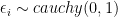
I decided on a Gaussian process model based on the following. After doing some exploratory analysis, I notice there was a clear non-linear effect between angle and hitspeed. Furthermore, there was heterogeneity for each hittype. For the non-linear effect, I decided on a GP, but similarly we could use a spline if the GP doesn’t scale. For the heterogeneity in different hittypes, I used a varying intercept. I ended up using a Cauchy prior, since after investigating the models posterior, posterior predictive distribution for each $latex fj$ placed too much mass around the functional mean of 0. The model can be written as follows:

But I prefer the following formulation. Since I centered and standardized the data, I omit a global intercept. Each 
![y_i = \beta_{j[i]} + f_{j[i]} + \epsilon_i](https://s0.wp.com/latex.php?latex=y_i+%3D+%5Cbeta_%7Bj%5Bi%5D%7D+%2B+f_%7Bj%5Bi%5D%7D+%2B+%5Cepsilon_i&bg=ffffff&fg=000&s=0&c=20201002)


And the Stan code is as follows:
writeLines(readLines("gp_regression_ard_linear.stan"));## functions {
##
## // these equations can be found in GPML
## vector gp_pred_rng(vector[] x_pred,
## vector y1, vector[] x,
## real magnitude, real[] length_scale,
## real sigma) {
## int N = rows(y1);
## int N_pred = size(x_pred);
## vector[N_pred] f2;
## {
## matrix[N, N] K = add_diag(gp_exp_quad_cov(x, magnitude, length_scale),
## sigma);
## matrix[N, N] L_K = cholesky_decompose(K);
## vector[N] L_K_div_y1 = mdivide_left_tri_low(L_K, y1);
## vector[N] K_div_y1 = mdivide_right_tri_low(L_K_div_y1', L_K)';
## matrix[N, N_pred] k_x_x_pred = gp_exp_quad_cov(x, x_pred, magnitude, length_scale);
## f2 = (k_x_x_pred' * K_div_y1);
## }
## return f2;
## }
## }
## data {
## int<lower=1> N;
## int<lower=1> D;
## vector[D] x[N];
## vector[N] y;
##
## // to generate posterior predictive for
## int<lower=1> N_pred;
## vector[D] x_pred_gb[N_pred];
## vector[D] x_pred_ld[N_pred];
## vector[D] x_pred_fb[N_pred];
## vector[D] x_pred_pu[N_pred];
## vector[D] x_pred_u[N_pred];
## }
## transformed data {
## vector[N] mu;
## mu = rep_vector(0, N);
## }
## parameters {
## // GP parameters
## real<lower=0> magnitude;
## real<lower=0> length_scale[D];
## vector[N] eta;
##
## // likelihood parameters
## real<lower=0> sigma;
## }
## transformed parameters {
## // latent f setup
## vector[N] f;
## {
## matrix[N, N] K;
## matrix[N, N] L_K;
## K = gp_exp_quad_cov(x, magnitude, length_scale);
## K = add_diag(K, .0001);
## L_K = cholesky_decompose(K);
## f = L_K * eta;
## }
## }
## model {
## magnitude ~ normal(0, 1);
## length_scale ~ normal(0, 1);
## eta ~ normal(0, 1);
##
## sigma ~ normal(0, 10);
##
## target += cauchy_lpdf(y | f, sigma);
## }
## generated quantities {
## vector[N_pred] y_pred_gb;
## vector[N_pred] y_pred_ld;
## vector[N_pred] y_pred_fb;
## vector[N_pred] y_pred_pu;
## vector[N_pred] y_pred_u;
##
## vector[N_pred] f_pred_gb = gp_pred_rng(x_pred_gb, y, x, magnitude, length_scale, sigma);
## vector[N_pred] f_pred_ld = gp_pred_rng(x_pred_ld, y, x, magnitude, length_scale, sigma);
## vector[N_pred] f_pred_fb = gp_pred_rng(x_pred_fb, y, x, magnitude, length_scale, sigma);
## vector[N_pred] f_pred_pu = gp_pred_rng(x_pred_pu, y, x, magnitude, length_scale, sigma);
## vector[N_pred] f_pred_u = gp_pred_rng(x_pred_u, y, x, magnitude, length_scale, sigma);
##
## for (n in 1:N_pred) y_pred_gb[n] = normal_rng(f_pred_gb[n], sigma);
## for (n in 1:N_pred) y_pred_ld[n] = normal_rng(f_pred_ld[n], sigma);
## for (n in 1:N_pred) y_pred_fb[n] = normal_rng(f_pred_fb[n], sigma);
## for (n in 1:N_pred) y_pred_pu[n] = normal_rng(f_pred_pu[n], sigma);
## for (n in 1:N_pred) y_pred_u[n] = normal_rng(f_pred_u[n], sigma);
## }In Sample Predictions, Smaller Model
csv = read_stan_csv("output_cauchy.csv");
samples = rstan::extract(csv);
## saved from an earlier session
y_sd = 10.7;
y_mu = 91.362
x_sd = 20.57;
x_mu = 9.35;
## unscale after sampling
samples$f_pred_gb = samples$f_pred_gb * y_sd + y_mu;
samples$f_pred_ld = samples$f_pred_ld * y_sd + y_mu;
samples$f_pred_fb = samples$f_pred_fb * y_sd + y_mu;
samples$f_pred_pu = samples$f_pred_pu * y_sd + y_mu;
samples$f_pred_u = samples$f_pred_u * y_sd + y_mu;
angle = seq(-3, 3, by = .05);
angle = angle * x_sd + x_mu;
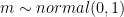
par(mfrow = c(2, 2));
f_gb_mu = colMeans(samples$f_pred_gb); ## ground ball mean function.
for(i in 1:1000) {
plot(angle, samples$f_pred_gb[i,], type = "l", col = "#092C5C", ylim = c(60, 120),
xaxt = "n", yaxt = "n", xlab = "", ylab ="", xlim = c(-60,75))
par(new = T);
}
plot(angle, f_gb_mu, type = "l", col = "#F5D130", ylim = c(60, 120), xlim = c(-60, 75),
xlab = "angle", ylab = "hitspeed", main = "ground ball");
f_ld_mu = colMeans(samples$f_pred_ld);
for(i in 1:1000) {
plot(angle, samples$f_pred_ld[i,], type = "l", col = "#092C5C", ylim = c(60, 120),
xaxt = "n", yaxt = "n", xlim = c(-60, 75), xlab = "", ylab = "");
par(new = T);
}
plot(angle, f_ld_mu, type = "l", col = "#F5D130", ylim = c(60, 120), xlab ="angle",
ylab = "hitspeed", main = "line drive", xlim = c(-60, 75));
f_fb_mu = colMeans(samples$f_pred_fb);
for(i in 1:1000) {
plot(angle, samples$f_pred_fb[i,], type = "l", col = "#092C5C", ylim = c(60, 120),
xaxt = "n", yaxt = "n", xlim = c(-60, 75), xlab = "", ylab = "");
par(new = T);
}
plot(angle, f_fb_mu, type = "l", col = "#F5D130", ylim = c(60, 120), xlab ="angle",
ylab = "hitspeed", main = "fast ball", xlim = c(-60, 75));
f_pu_mu = colMeans(samples$f_pred_pu);
for(i in 1:1000) {
plot(angle, samples$f_pred_pu[i,], type = "l", col = "#092C5C", ylim = c(60, 120),
xaxt = "n", yaxt = "n", xlim = c(-60, 75), xlab = "", ylab = "");
par(new = T);
}
plot(angle, f_pu_mu, type = "l", col = "#F5D130", ylim = c(60, 120), xlab ="angle",
ylab = "hitspeed", main = "pop up", xlim = c(-60, 75));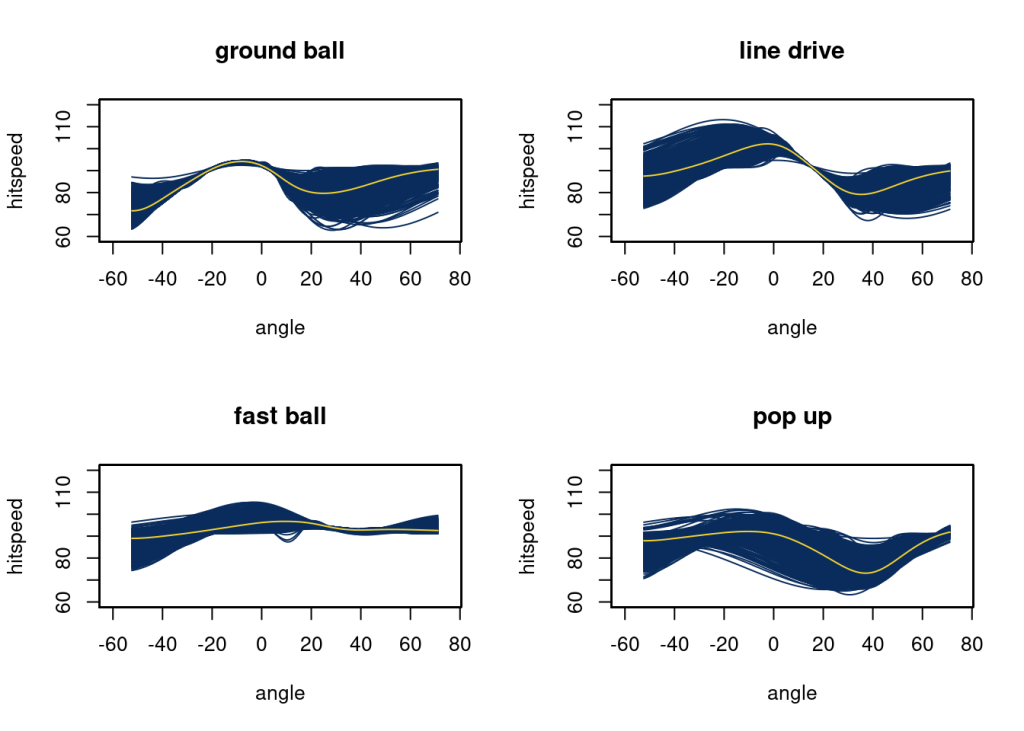
# f_u_mu = colMeans(samples$f_pred_u);
# for(i in 1:1000) {
#   plot(angle, samples$f_pred_u[i,], type = "l", col = "#092C5C", ylim = c(60, 120),
#        xaxt = "n", yaxt = "n", xlim = c(-60, 75), xlab = "", ylab = "");
#   par(new = T);
# }
# plot(angle, f_u_mu, type = "l", col = "#F5D130", ylim = c(60, 120), xlab ="angle",
#      ylab = "hitspeed", main = "u", xlim = c(-60, 75))
At higher angles, the popup will have less speed. Anything below an angle of 20 for the line drive will have a higher speed. Ground balls have a higher speed around an angle of -10.
Larger Model
csv = read_stan_csv("output_larger_cauchy_final.csv");
samples = rstan::extract(csv);


## unscale after sampling
samples$f_pred_gb = samples$f_pred_gb * y_sd + y_mu;
samples$f_pred_ld = samples$f_pred_ld * y_sd + y_mu;
samples$f_pred_fb = samples$f_pred_fb * y_sd + y_mu;
samples$f_pred_pu = samples$f_pred_pu * y_sd + y_mu;
samples$f_pred_u = samples$f_pred_u * y_sd + y_mu;
angle = seq(-3, 3, by = .05);
angle = angle * x_sd + x_mu;

par(mfrow = c(2, 2));
f_gb_mu = colMeans(samples$f_pred_gb);  ## ground ball mean function.
for(i in 1:1000) {
  plot(angle, samples$f_pred_gb[i,], type = "l", col = "#092C5C", ylim = c(60, 120),
       xaxt = "n", yaxt = "n", xlab = "", ylab ="", xlim = c(-60,75))
  par(new = T);
}
plot(angle, f_gb_mu, type = "l", col = "#F5D130", ylim = c(60, 120), xlim = c(-60, 75),
     xlab = "angle", ylab = "hitspeed", main = "ground ball");

f_ld_mu = colMeans(samples$f_pred_ld);
for(i in 1:1000) {
  plot(angle, samples$f_pred_ld[i,], type = "l", col = "#092C5C", ylim = c(60, 120),
       xaxt = "n", yaxt = "n", xlim = c(-60, 75), xlab = "", ylab = "");
  par(new = T);
}
plot(angle, f_ld_mu, type = "l", col = "#F5D130", ylim = c(60, 120), xlab ="angle",
     ylab = "hitspeed", main = "line drive", xlim = c(-60, 75));

f_fb_mu = colMeans(samples$f_pred_fb);
for(i in 1:1000) {
  plot(angle, samples$f_pred_fb[i,], type = "l", col = "#092C5C", ylim = c(60, 120),
       xaxt = "n", yaxt = "n", xlim = c(-60, 75), xlab = "", ylab = "");
  par(new = T);
}
plot(angle, f_fb_mu, type = "l", col = "#F5D130", ylim = c(60, 120), xlab ="angle",
     ylab = "hitspeed", main = "fast ball", xlim = c(-60, 75));

f_pu_mu = colMeans(samples$f_pred_pu);
for(i in 1:1000) {
  plot(angle, samples$f_pred_pu[i,], type = "l", col = "#092C5C", ylim = c(60, 120),
       xaxt = "n", yaxt = "n", xlim = c(-60, 75), xlab = "", ylab = "");
  par(new = T);
}
plot(angle, f_pu_mu, type = "l", col = "#F5D130", ylim = c(60, 120), xlab ="angle",
     ylab = "hitspeed", main = "pop up", xlim = c(-60, 75));
# f_u_mu = colMeans(samples$f_pred_u);
# for(i in 1:1000) {
#   plot(angle, samples$f_pred_u[i,], type = "l", col = "#092C5C", ylim = c(60, 120),
#        xaxt = "n", yaxt = "n", xlim = c(-60, 75), xlab = "", ylab = "");
#   par(new = T);
# }
# plot(angle, f_u_mu, type = "l", col = "#F5D130", ylim = c(60, 120), xlab ="angle",
#      ylab = "hitspeed", main = "u", xlim = c(-60, 75))
Here, as expected, we get more complex functions as the dataset grows. Ground balls now have a more steadily increasing speed from -40 to 0 degrees. The speed off bat of a line drive decreased quickly at higher angles. Fast balls are similar at all angles. Speed off bat for popups drops off after 0 and returns to about 90 at an angle of 60.

Leave a comment