likely llc

Dr. Murthy and I have been working on a way to interpret omics data. We’d like to see if there’s any natural grouping structure to a large dataset. We’ve computed something resembling a cross covariance matrix. After Dr. Murthy experimented with sparse CCA for a while, we tried some other clustering methods or regularization methods with marginal results.

After doing some thinking, I realized we could probably just rely on good-old singular value decomposition. As happens a lot in applied statistics, machine learning, and data science, we can usually just use traditional applied mathematics or statistics methods, and don’t need anything fancy. I’ll show you what I’m talking about.

When we’re trying to figure out if a method works, we usually simulate data. First, after loading some packages, I simulate several rows of a matrix that are generated from normal distributions with different means, here:

N = 20;
M = 10;
A = matrix(NA, nrow = N, ncol = M);
A[1:8,] = rnorm(M * 8, 2, 1);
A[9:14,] = rnorm(M * 6, 0, .5);
A[15:N,] = rnorm(M * 6, 5, 1);

Next, we take a look at a heatmap to see if the structure looks as intended:

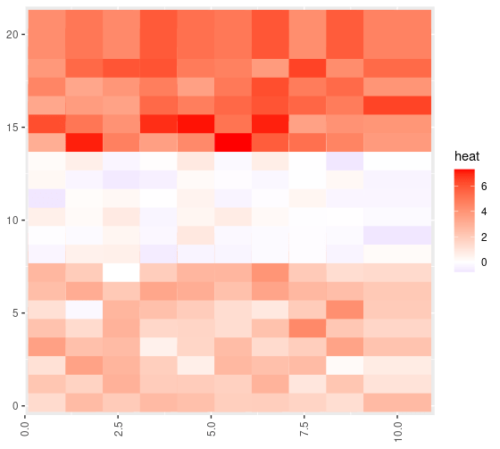
Looks good to me.


Next, we randomly permute the rows of the matrix, as if the data we’ve observed has no particular structure. Here’s the code:

A = matrix(NA, nrow = N, ncol = M);
re_order = sample(1:N);
for (j in 1:M) {
  A[, j] = A_original[, j][re_order];
}

Here’s the heatmap of the randomly permuted matrix:

Looking at a raw heatmap of the observed data, we can see it might not look like there’s any intended structure. But we can find some structure with SVD. Let’s take the SVD of the matrix A:

We check out the first left eigenvector, , sort it, and make a plot. Here’s the code for what I’m talking about, starting from the SVD, extracting the first left eigenvector, sorting it, and making the plot:

tmp_svd_A = svd(A);
U = tmp_svd_A$u;

U1 = U[,1];
U1_order = order(U1, decreasing = T);
U1_sorted = U1[U1_order];

plot(1:20, U1_sorted, xlab = "index", ylab = "u1 sorted")

We can then plot the sorted, first, left, eigenvector. We’re looking for big gaps.

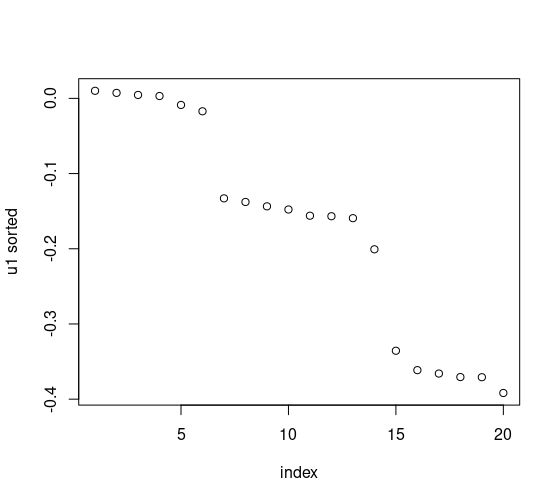
There’s pretty clearly 3 clear clusters, after the 6th observation, and after the 14th. If we really wanted to, we could project onto the y-axis, but that’s overkill.

We can explicitly compute the difference of all the values in the first left eigenvector, and choose the top N clusters, and compute the cluster labels if you’d like. We can do that with something like the following code, with 3 clusters:

diffi = abs(diff(Uj_sorted));
largest_diffs = sort(which.maxn(diffi, n = 3 - 1));
clusters = c(rep(1, largest_diffs[1]), 
             rep(2, largest_diffs[2] - largest_diffs[1]),
             rep(3, N - largest_diffs[2]));

To recover this structure in the original matrix, we simply re-order each column with the ordering of the first eigenvector. Here’s the code:

A_reordered = matrix(NA, nrow = N, ncol = M);
for (j in 1:M) {
  A_reordered[, j] = A[, j][U1_order];
}

And here’s what the final heatmap looks like:

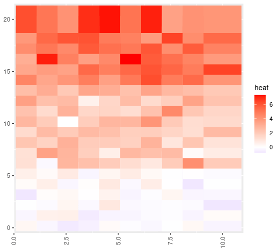
We’ve recovered the simulated structure, with minimal code. There’s more you can do with this simple method. Soon, you’ll see this applied on a the real data, but with some more bells and whistles. Full R code below, didn’t clean it up. Enjoy!

library(doBy);
library(ggplot2);
set.seed(1);

N = 20;
M = 10;
A = matrix(NA, nrow = N, ncol = M);
A[1:8,] = rnorm(M * 8, 2, 1);
A[9:14,] = rnorm(M * 6, 0, .5);
A[15:N,] = rnorm(M * 6, 5, 1);


## plot original A
df = expand.grid(x = 1:N, y = 1:M);
df = cbind(df, as.vector(A));
colnames(df)[3] = "heat";
p = ggplot(df, aes(x, y)) + geom_tile(aes(colour = heat), size = 12) + 
  scale_color_gradient2(low = "blue",
                        high = "red", mid = "white")  + 
  theme(axis.title=element_blank(), 
        axis.text.x=element_text(angle=90, hjust=1, vjust=0.5)) + 
  coord_equal() + coord_flip();
p

A_original = A;

## perturb each row
A = matrix(NA, nrow = N, ncol = M);

## properly re-ordered
re_order = sample(1:N);
for (j in 1:M) {
  A[, j] = A_original[, j][re_order];
}

## plot re-ordered A
df = expand.grid(x = 1:N, y = 1:M);
df = cbind(df, as.vector(A));
colnames(df)[3] = "heat";
p = ggplot(df, aes(x, y)) + geom_tile(aes(colour = heat), size = 12) + 
  scale_color_gradient2(low = "blue",
                        high = "red", mid = "white")  + 
  theme(axis.title=element_blank(), 
        axis.text.x=element_text(angle=90, hjust=1, vjust=0.5)) + 
  coord_equal() + coord_flip();
p

## now we try re-ordering based on the first principal component
tmp_svd_A = svd(A);
U = tmp_svd_A$u;
V = tmp_svd_A$v;
svs = tmp_svd_A$d;

j = 1;
Uj = U[,j];
Uj_order = order(Uj, decreasing = T); ## this is to find biggest gaps
Uj_sorted = Uj[Uj_order];
diffi = abs(diff(Uj_sorted));
largest_diffs = sort(which.maxn(diffi, n = k - 1));
clusters = c(rep(1, largest_diffs[1]), 
             rep(2, largest_diffs[2] - largest_diffs[1]),
             rep(3, N - largest_diffs[2]));

## re-order A
A_reordered = matrix(NA, nrow = N, ncol = M);
for (j in 1:M) {
  A_reordered[, j] = A[, j][Uj_order];
}


## plot the re-ordered A again
df = expand.grid(x = 1:N, y = 1:M);
df = cbind(df, as.vector(A_reordered));
colnames(df)[3] = "heat";
p = ggplot(df, aes(x, y)) + geom_tile(aes(colour = heat), size = 12) + 
  scale_color_gradient2(low = "blue",
                        high = "red", mid = "white")  + 
  theme(axis.title=element_blank(), 
        axis.text.x=element_text(angle=90, hjust=1, vjust=0.5)) + 
  coord_equal() + coord_flip();
p