Additive Gaussian Process Time Series Regression in Stan

I’ve copied this over from discourse.mc-stan.org, but this was my post, so I’m comfortable doing so.

While working in the psychiatry department at Michigan, I played around with EEG data. Next, I became curious about how to extract out different periodic components of a time series. I ended up finding a blog post on Andrew Gelman’s blog, and found a statistical model, we call the birthday problem, by Professor Vehtari, that did exactly that. Later, in 2018, he allowed me work an internship at Aalto University, implementing parts of the Gaussian process library for the Stan math library. Here’s a simplified version of how to build this model in Stan, using Gaussian processes.

Suppose, first, that we have some observed time series $y$ , that’s additive of two signals, $f_1$ and $f_2$ , and some noise, $\epsilon$ . In math, that’s

$y(x) = f_1(x) + f_2(x) + \epsilon$

And, for simplicity, we set $y$ to be the sum of a linear function, $f_1$ , and a sine wave $f_2$ . I did some re-scaling so the function looked like I wanted it to. That’s

$f_1(x) = 2x$

$f_2(x) = sin(\frac{x}{2\pi})$

And this can be implemented and dumped into a file to be read into cmdstan as follows, in R.

N=100;
D=1;
x = as.matrix(1:N);
x_pred = as.matrix(seq(0,100, length.out = 1000));
N_pred = as.vector(length(x_pred));
y1 = 2 * x;
y2 = sin(x / (2*pi))
y1 = (y1 - mean(y1)) / (sd(x));
y2 = y2 - mean(y2);
y_obs = y1 + y2 + rnorm(N, 0, .25);
y = as.vector(y_obs - mean(y_obs));

stan_rdump(c("x", "y", "N", "D", "x_pred", "N_pred"), "gp_simu_ts.data.R")

Which, when plotted in base R, looks as follows.

Looks like some structure. What if, for example, we’re modeling global warming, and we want to see, on average, the linear increase in temperature over time, adjusting for periodicity, (i.e. seasonal effects)? We can use Gaussian process regression to do so.

In order to recover this signal, I’m going to use a linear kernel, and a squared exponential. In layman’s terms, I’m assuming that there’s some linear effect, and some smooth effect which I can’t really assume the shape of. I should use a periodic kernel, but this required some debugging in C++ that I didn’t have time to do. The model becomes

$f_1(x) \sim GP(0, k_1), k_1(x, x') = \sigma_1^2 exp(\frac{d(x, x')^2}{l_1^2})$

$f_2(x) \sim GP(0, k_2), k_2(x, x') = \sigma_2^2 (x, x')$

for $d(x, x')$ , Euclidean distance, and $(x, x')$ the inner product, using notation from functional analysis.

We can compute the total covariance matrix, in an additive model, by summing the two covariance matrices. That’s

$k_{tot} = k_1 + k_2$ .

If we want to make posterior predictive predictions, for the mean function, we can use the following formula.

$\bar{f} = k (k + I \sigma^2)^{-1}y$

But say we only want to make predictions for the linear kernel, or more generally, if we sum a few kernels, predictions for $f_{\gamma}$ . We can compute that using following:

$\bar{f}_{\gamma} = k_{\gamma} (k_{tot} + I \sigma^2)^{-1}y$

The snipped of Stan code, where we’re making posterior predictions, is implemented in the functions block, and is as follows.

 vector gp_pred_dot_prod_rng(vector[] x2,
                              vector y, vector[] x1,
                              real m, real l,
                              real sig,
                              real sigma) {
    int N1 = rows(y);
    int N2 = size(x2);
    vector[N2] f;
    {
      matrix[N1, N1] K = add_diag(gp_exp_quad_cov(x1, m, l) +
                                  gp_dot_prod_cov(x1, sig), sigma);
      matrix[N1, N1] L_K = cholesky_decompose(K);
      vector[N1] L_K_div_y = mdivide_left_tri_low(L_K, y);
      vector[N1] K_div_y = mdivide_right_tri_low(L_K_div_y', L_K)';
      matrix[N1, N2] k_x1_x2 = gp_dot_prod_cov(x1, x2, sig);
      f = (k_x1_x2' * K_div_y);
    }
    return f;
  }

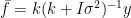
And here’s predictions for $f_1$ :

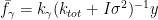
And here’s predictions for $f_2$ :

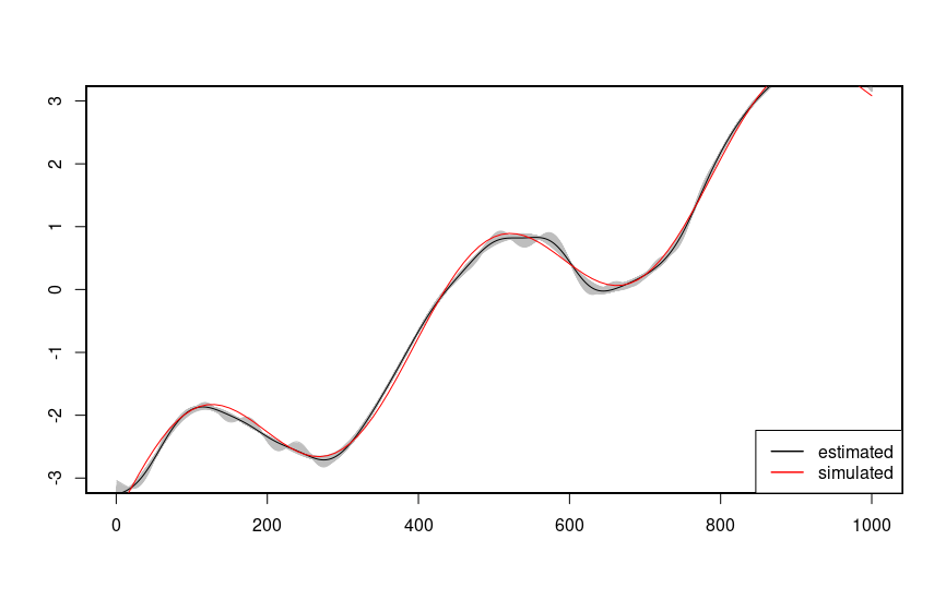
And the total additive model:

Here’s a link to the original discourse post: https://discourse.mc-stan.org/t/gaussian-process-out-of-sample-predictive-distribution/16891/11. Initially, we were discussing making posterior predictions when working with Gaussian process models. I’ve since deleted that account, but you’ve any doubt I wrote this post, you can contact Professor Vehtari or the other Stan developers.

And here’s all of the code, beginning with the Stan code, and after with the R code.

functions {
  vector gp_pred_exp_quad_rng(vector[] x2,
                              vector y, vector[] x1,
                              real m, real l,
                              real sig,
                              real sigma) {
    int N1 = rows(y);
    int N2 = size(x2);
    vector[N2] f;
    {
      matrix[N1, N1] K = add_diag(gp_exp_quad_cov(x1, m, l) +
                                  gp_dot_prod_cov(x1, sig), sigma);
      matrix[N1, N1] L_K = cholesky_decompose(K);
      vector[N1] L_K_div_y = mdivide_left_tri_low(L_K, y);
      vector[N1] K_div_y = mdivide_right_tri_low(L_K_div_y', L_K)';
      matrix[N1, N2] k_x1_x2 = gp_exp_quad_cov(x1, x2, m, l);
      f = (k_x1_x2' * K_div_y);
    }
    return f;
  }
  vector gp_pred_dot_prod_rng(vector[] x2,
                              vector y, vector[] x1,
                              real m, real l,
                              real sig,
                              real sigma) {
    int N1 = rows(y);
    int N2 = size(x2);
    vector[N2] f;
    {
      matrix[N1, N1] K = add_diag(gp_exp_quad_cov(x1, m, l) +
                                  gp_dot_prod_cov(x1, sig), sigma);
      matrix[N1, N1] L_K = cholesky_decompose(K);
      vector[N1] L_K_div_y = mdivide_left_tri_low(L_K, y);
      vector[N1] K_div_y = mdivide_right_tri_low(L_K_div_y', L_K)';
      matrix[N1, N2] k_x1_x2 = gp_dot_prod_cov(x1, x2, sig);
      f = (k_x1_x2' * K_div_y);
    }
    return f;
  }
  vector gp_pred_rng(vector[] x2,
                              vector y, vector[] x1,
                              real m, real l,
                              real sig,
                              real sigma) {
    int N1 = rows(y);
    int N2 = size(x2);
    vector[N2] f;
    {
      matrix[N1, N1] K = add_diag(gp_exp_quad_cov(x1, m, l) +
                                  gp_dot_prod_cov(x1, sig), sigma);
      matrix[N1, N1] L_K = cholesky_decompose(K);
      vector[N1] L_K_div_y = mdivide_left_tri_low(L_K, y);
      vector[N1] K_div_y = mdivide_right_tri_low(L_K_div_y', L_K)';
      matrix[N1, N2] k_x1_x2 = gp_exp_quad_cov(x1, x2, m, l) +
	gp_dot_prod_cov(x1, x2, sig);
      f = (k_x1_x2' * K_div_y);
    }
    return f;
  }
}
data {
  int<lower=1> N;
  int<lower=1> D;
  vector[D] x[N];
  vector[N] y;

  int<lower=1> N_pred;
  vector[D] x_pred[N_pred];
}
transformed data {
  vector[N] mu = rep_vector(0, N);
}
parameters {
  real<lower=0> l;
  real<lower=0> m;
  real<lower=0> sig0;

  real<lower=0> sigma;
}
transformed parameters {
  matrix[N, N] L_K;
  {
    matrix[N, N] K = gp_exp_quad_cov(x, m, l) + gp_dot_prod_cov(x, sig0);
    
    K = add_diag(K, sigma);
    L_K = cholesky_decompose(K);
  }
}
model {
  m ~ normal(0, 1);
  l ~ normal(0, 1);
  sig0 ~ normal(0, 1);

  sigma ~ normal(0, 1);
  
  y ~ multi_normal_cholesky(mu, L_K);
}
generated quantities {
  vector[N_pred] f1_pred = gp_pred_exp_quad_rng(x_pred, y, x, m, l,
                                           sig0, sigma);
  vector[N_pred] f2_pred = gp_pred_dot_prod_rng(x_pred, y, x, m, l,
                                           sig0, sigma);
  vector[N_pred] f3_pred = gp_pred_rng(x_pred, y, x, m, l,
                                           sig0, sigma);
}

setwd("/home/andre/stan_discourse/");
require(rstan);


N=100;
D=1;
x = as.matrix(1:N);
x_pred = as.matrix(seq(0,100, length.out = 1000));
N_pred = as.vector(length(x_pred));
y1 = 2 * x;
y2 = sin(x / (2*pi))
y1 = (y1 - mean(y1)) / (sd(x));
y2 = y2 - mean(y2);
y_obs = y1 + y2 + rnorm(N, 0, .25);
y = as.vector(y_obs - mean(y_obs));



stan_rdump(c("x", "y", "N", "D", "x_pred", "N_pred"), "gp_simu_ts.data.R")

csv = read_stan_csv("output.csv")
samples = rstan::extract(csv);

for (i in 1:1000){
  plot(samples$f1_pred[i,], xlim=c(0,1000), ylim = c(-3,3), type = "l", yaxt = "n", xaxt = "n", xlab = "", ylab = "", col = "grey")
  par(new = T)
}
plot(colMeans(samples$f1_pred), xlim=c(0,1000), ylim = c(-3, 3), type = "l", xlab = "", ylab = "");
par(new = T);
plot(x, y2, ylim =c(-3,3), xlim = c(0,100), xaxt = "n", yaxt="n", xlab = "", ylab = "", type = "l", col = "red");
legend("bottomright", c("estimated", "simulated"), lwd = c(1.5, 1.5), col = c("black", "red"))

for (i in 1:1000){
  plot(samples$f2_pred[i,], xlim=c(0,1000), ylim = c(-3,3), type = "l", yaxt = "n", xaxt = "n", xlab = "", ylab = "", col = "grey")
  par(new = T)
}
plot(colMeans(samples$f2_pred), xlim=c(0,1000), ylim = c(-3, 3), type = "l", xlab = "", ylab = "");
par(new = T);
plot(x, y1, ylim =c(-3,3), xlim = c(0,100), xaxt = "n", yaxt="n", xlab = "", ylab = "",  type = "l", col = "red");
legend("bottomright", c("estimated", "simulated"), lwd = c(1.5, 1.5), col = c("black", "red"))


for (i in 1:1000){
  plot(samples$f3_pred[i,], xlim=c(0,1000), ylim = c(-3,3), type = "l", yaxt = "n", xaxt = "n", xlab = "", ylab = "", col = "grey")
  par(new = T)
}
plot(colMeans(samples$f3_pred), xlim=c(0,1000), ylim = c(-3, 3), type = "l", xlab = "", ylab = "");
par(new = T);
plot(x, y1 + y2, ylim =c(-3,3), xlim = c(0,100), xaxt = "n", yaxt="n", xlab = "", ylab = "", col = "red", type = "l");
legend("bottomright", c("estimated", "simulated"), lwd = c(1.5, 1.5), col = c("black", "red"))

One response to “Additive Gaussian Process Time Series Regression in Stan”

What happened at Aalto University. Internship Summer 2018 (Part 1). – likely llc

August 24, 2022 at 4:42 am

[…] what’s known as “the birthday problem” in Stan. It’s similar to this post: https://likelyllc.com/2022/08/03/additive-gaussian-process-time-series-regression-in-stan/, but with a few caveats. Take a look at BDA3, page 505, section 21.2, for a more rigorous […]

LikeLike

likely llc