likely llc

For Michigan, I’ve since applied the SVD based sorting algorithm, which can be used for clustering, to real data. The goal is to in some way model the relationship of proteins and metabolites, come up with modules, or groups of proteins and metabolites that were related, and then use these later in a regression model to see which groups are associated with outcomes such as cardiovascular disease (CVD) or cholesterol.

The data here is something like this. Suppose, for example, we have proteins, patients and metabolites. The protein and metabolite, matrix are then and respectively. For this next step, recall the definition of covariance. Suppose we have matrices and . The definition is as follows, where is the mathematical expectation.

We do something similar to render a protein-metabolite cross covariance matrix. That is, we scale (or standardize) the matrix by each row, for , along the protein axis, and each column, for along the metabolite axis. After, scaling, we take the inner product, we get a matrix I’ll call , which is as follows.

The cross-covariance matrix looks like this.

What a mess!

Next, we’d like to determine if there’s any modules, as we’ve done in the previous post on simulated data, which can be found here: https://likelyllc.com/2022/06/13/using-svd-for-clustering/. In this case, we sort by using both the first, left, singular vector and first, right singular vector. The code snippets are below, with full code to follow. Remember to sort the names as well, so the plot renders with the correct names!

# order by first left singular vector
K_ab_svd_tmp = svd(K_ab);
U = K_ab_svd_tmp$u;
Uj = U[,j];
Uj_order = order(Uj, decreasing = T); 
Uj_sorted = Uj[Uj_order];

K_ab_reordered = matrix(NA, nrow = nrow(K_ab), ncol = ncol(K_ab));
for (j in 1:ncol(K_ab)) {
  K_ab_reordered[, j] = K_ab[,j][Uj_order];
}
prot_names = prot_names[Uj_order];

# order by first right singular vector
K_ab_svd_re_ordered_tmp = svd(K_ab_reordered);
V = K_ab_svd_re_ordered_tmp$v;
Vti = Vt[i,];
Vti_order = order(Vti, decreasing = T);
Vti_sorted = Vti[Vti_order];
K_ab_reordered_2 = matrix(NA, nrow = nrow(K_ab), ncol = ncol(K_ab));
for (i in 1:nrow(K_ab)) {
  K_ab_reordered_2[i, ] = K_ab_reordered[i,][Vti_order];
}
meta_names = meta_names[Vti_order];

Recall this diagnostic plot from the previous post, where we can see there are three clear clusters, on simulated data:

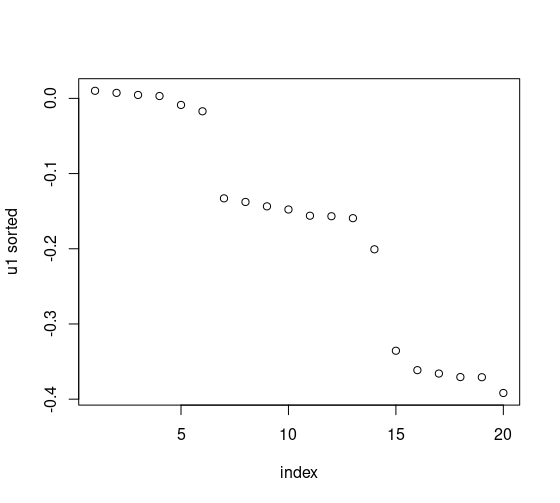
Let’s take a look at these plots but for metabolites and proteins. We can compute the differences, explicitly, too.

Looks like there are no clear clusters, as determined by singular gaps, for the proteins, however, looks like we can see about 3 clusters for the proteins, depending on how you’d like to define them. For the former, this happens sometimes with real data! Although we like to categorize, sometimes in real life this isn’t possible. Furthermore, we can compute these explicitly.

After sorting using this strategy, we get the following plot. This, in my opinion, is a lot more easy to interpret than clustering using hierarchical clustering.

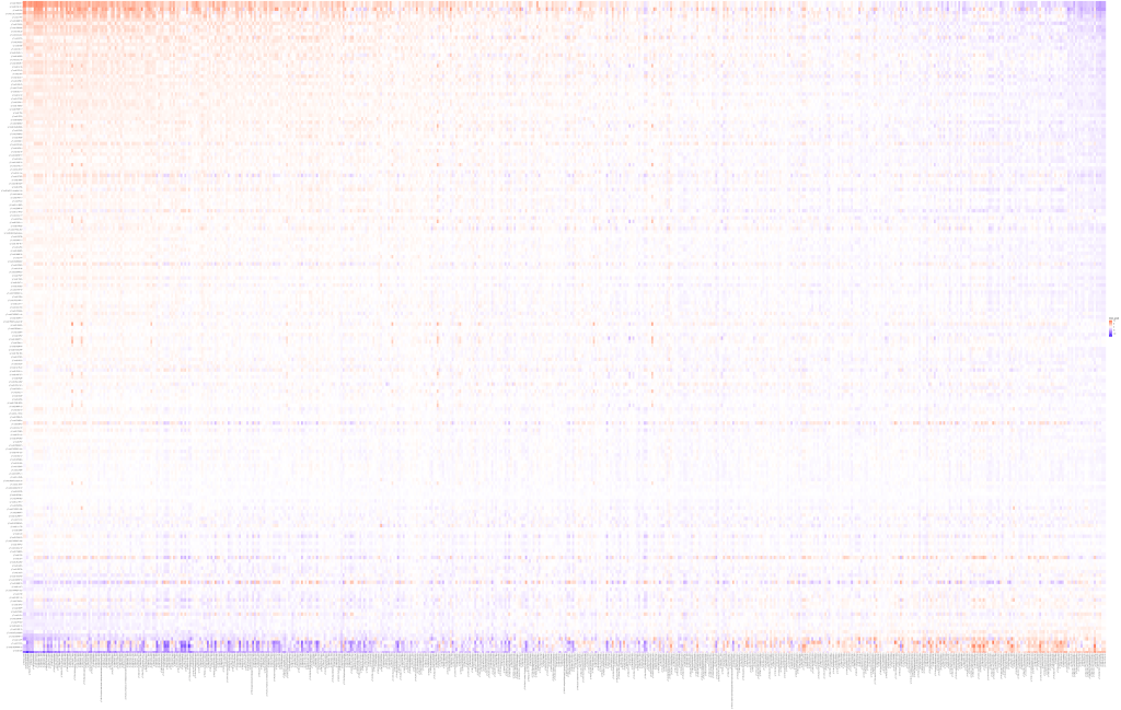
Full code below.

## now we use the spectral sorting on the real data with K_ab
library(doBy);
library(ggplot2);
set.seed(1);

setwd("/home/andre/venk/svd_clustering/");
load("for_andre.RData");


df = expand.grid(x = 1:N, y = 1:M);
df = cbind(df, as.vector(K_ab));
colnames(df)[3] = "inner_prod";
p = ggplot(df, aes(x, y)) + geom_tile(aes(colour = inner_prod), size = 12) + 
  scale_color_gradient2(low = "blue",
                        high = "red", mid = "white")  + 
  theme(axis.title=element_blank(), 
        axis.text.x=element_text(angle=90, hjust=1, vjust=0.5)) + 
  coord_equal() + coord_flip() + theme(legend.position = "none");
p

K_ab_svd_tmp = svd(K_ab);
U = K_ab_svd_tmp$u;
V = K_ab_svd_tmp$v;
svds = K_ab_svd_tmp$d;

prot_names = rownames(K_ab);
meta_names = colnames(K_ab);



j = 1;
k = 3;
Uj = U[,j];
Uj_order = order(Uj, decreasing = T); ## this is to find biggest gaps
Uj_sorted = Uj[Uj_order];
diffi = abs(diff(Uj_sorted));
largest_diffs = sort(which.maxn(diffi, n = k - 1));
# clusters = c(rep(1, largest_diffs[1]), 
#              rep(2, largest_diffs[2] - largest_diffs[1]),
#              rep(3, N - largest_diffs[2]));

K_ab_reordered = matrix(NA, nrow = nrow(K_ab), ncol = ncol(K_ab));
for (j in 1:ncol(K_ab)) {
  K_ab_reordered[, j] = K_ab[,j][Uj_order];
}
prot_names = prot_names[Uj_order];

N = nrow(K_ab);
M = ncol(K_ab);

df = expand.grid(x = 1:N, y = 1:M);
df = cbind(df, as.vector(K_ab_reordered));
colnames(df)[3] = "inner_prod";
p = ggplot(df, aes(x, y)) + geom_tile(aes(colour = inner_prod), size = 12) + 
  scale_color_gradient2(low = "blue",
                        high = "red", mid = "white")  + 
  theme(axis.title=element_blank(), 
        axis.text.x=element_text(angle=90, hjust=1, vjust=0.5)) + 
  coord_equal() + coord_flip();
p

## now we try the row sorting as well
## we'll take a leap and do it for
K_ab_svd_re_ordered_tmp = svd(K_ab_reordered);
U = K_ab_svd_re_ordered_tmp$u;
V = K_ab_svd_re_ordered_tmp$v;
svds = K_ab_svd_re_ordered_tmp$d;

i = 1;
Vt = t(V);
Vti = Vt[i,];
Vti_order = order(Vti, decreasing = T);
Vti_sorted = Vti[Vti_order];
plot(Vti_sorted);

K_ab_reordered_2 = matrix(NA, nrow = nrow(K_ab), ncol = ncol(K_ab));
for (i in 1:nrow(K_ab)) {
  K_ab_reordered_2[i, ] = K_ab_reordered[i,][Vti_order];
}
meta_names = meta_names[Vti_order];

df = expand.grid(x = prot_names, y = meta_names);
df = cbind(df, as.vector(K_ab_reordered_2));
colnames(df)[3] = "inner_prod";
p = ggplot(df, aes(x, y)) + geom_tile(aes(colour = inner_prod), size = 12) + 
  scale_color_gradient2(low = "blue",
                        high = "red", mid = "white")  + 
  theme(axis.title=element_blank(), 
        axis.text.x=element_text(angle=90, hjust=1, vjust=0.5)) + 
  coord_equal() + coord_flip();
p

Edit: When solving a system of linear equations, we can only use row operations. Here, since, we’re not solving a system of linear equations, we need not worry about preserving the kernel. I’ll come back to this.